Tides and the sea level - Part 2

Two weeks ago we calculated the sea level elevation in Stavanger related to tidal motions given the amplitudes, periods and phases of 6 components. We are getting back to that example again, but now we will take a look at some observed data.

Task 1: First things first, we read from the dataset stavanger.txt. For this, we use the function read_csv from Pandas:

import pandas as pd

df = pd.read_csv('stavanger.txt', sep=r"\s+")

df.keys()

This gives us the following output:

Index(['time', 'ssh', 'anomaly', 'M2', 'S2', 'N2', 'K2', 'O1', 'K1', 'tide'], dtype='object')

The df Dataframe contains hourly dates between 09/2018 and 09/2019 of the observed sea surface height (cm) in Stavanger, its anomaly (ssh - mean) and the tidal elevations (of each component and their summation) that we calculated previously.

Task 2: To proceed with the comparison between the tidal components and the observed sea surface height, let’s select the first 45 days of the df dataset.

Tip: use the function iloc from Pandas.

import numpy as np

t = np.arange(0, 45*24+1, 1) # 45 days
df_sm = df.iloc[0:len(t)]

df_sm

We get the following output:

	time	ssh	anomaly	M2	S2	N2	K2	O1	K1	tide
2018-09-13	00:00:00	106.2	40.428946	14.966470	6.650923	1.380173	1.128245	1.367263	1.099229	26.592303
2018-09-13	01:00:00	105.3	39.528946	15.634982	5.426019	2.258865	1.173072	1.174997	0.745735	26.413670
2018-09-13	02:00:00	92.5	26.728946	12.386691	2.747218	2.592491	0.902034	0.913493	0.341124	19.883051
2018-09-13	03:00:00	88.4	22.628946	6.035344	-0.667698	2.300545	0.388111	0.598161	-0.086869	8.567594
2018-09-13	04:00:00	79.9	14.128946	-1.827951	-3.903705	1.453475	-0.230316	0.247583	-0.508908	-4.769821
...	...	...	...	...	...	...	...	...	...	...
2018-10-27	20:00:00	49.2	-16.571054	-13.860386	-2.747218	1.269579	0.628035	-0.076464	1.341275	-13.445178
2018-10-27	21:00:00	50.4	-15.371054	-8.388605	0.667698	2.192932	1.052723	0.288132	1.050467	-3.136652
2018-10-27	22:00:00	54.5	-11.271054	-0.815350	3.903705	2.587127	1.193952	0.635750	0.687655	8.192839
2018-10-27	23:00:00	66.2	0.428946	6.962163	6.093717	2.357046	1.013693	0.945905	0.277707	17.650232
2018-10-28	00:00:00	80.4	14.628946	12.995547	6.650923	1.558206	0.560485	1.200323	-0.151276	22.814208

1081 rows × 10 columns

Task 3: Let’s visualize how things look like. Plot the anomaly and tide variables.

import matplotlib.pyplot as plt

plt.plot(df_sm.anomaly.values, 'k--', label='Anomaly');
plt.plot(df_sm.tide.values, 'r-', label='Tides');

plt.legend(loc='upper right')
plt.show()

We get the following plot:

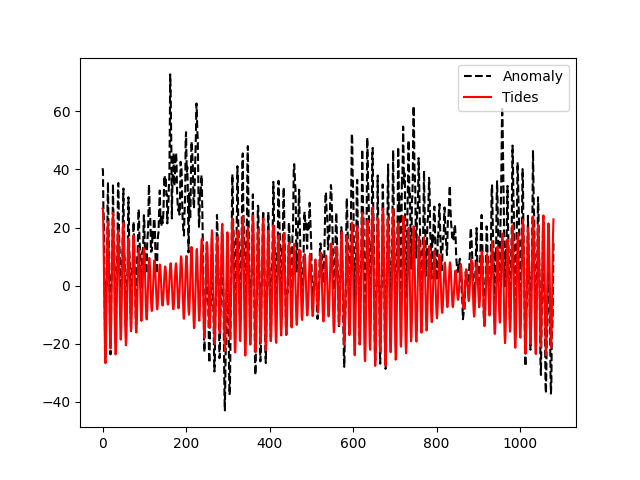
Very good! As expected (why?), the observed sea surface height is not equal to the pure tide signal, but if you zoom in at the peaks (or throughs), you will see that they are in phase and this is an indicator that we are on the right track.

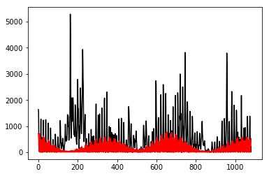
Question: How much of the observed signal is composed by tides?

To answer this, we will estimate the energy (J) contained in both signals by using the following equation:

\[E = \sum_{n=0}^{N} |F(t)|^2,\]

where N is the number of points of your signal (length) and F(t) is your time series.

Task 4: Given the previous equation, we calculate the energy of the anomaly and tide signals and the ratio between them. We implement the function energy that takes as arguments both signals and returns the \(\frac{E_{tide}}{E_{anomaly}}\) ratio as percentage.

def energy(anomaly, tide):
    e_anom = ((abs(anomaly))**2)
    e_tide = ((abs(tide))**2)

    # plot energies
    plt.plot(e_anom, 'k', e_tide,'r')

    ratio = np.sum(e_tide) / np.sum(e_anom) # calculate the ratio between the energies

    return ratio*100 # in percentage


# calculate the ratio
ratio = energy(df_sm.anomaly.values, df_sm.tide.values)

plt.show()

print('The ratio is: %f%%\n'%(ratio))

We get the following output:

The ratio is: 32.158691%

and the following plot:

As any other wave, tides also travel (propagate) in the ocean. Their phase velocity is given by:

\[c = \sqrt{(g*D)}\]

where g is the acceleration of gravity and D is the ocean depth.

Task 5: Considering g = 10 m s\(^{-2}\) and D = 4000 m, how fast (in m s\(^{-1}\)) does this wave travel?

How much time (in hours) does it take to travel from Stavanger to Bodø? Consider the distance between the two cities as 1200 km.

g = 10 # gravity
D = 4000 # water depth
L = 1200 # distance, in meters

c = (g*D)**0.5
print('The phase velocity is %f m/s'%(c))

dt = L/(c*3.6)
print('The phase velocity is %f hours'%(dt))

We get the following output:

The phase velocity is 200.000000 m/s
The phase velocity is 1.666667 hours

This is impressively fast, right? Putting these numbers in words, a tidal crest observed in Stavanger is also observed in Bodø, 1200 km away, a bit more than one and a half hours later!