Amospheric pressure and correlations
Let’s take another geosciences application. Here we will explore how the atmospheric pressure is related to environmental variables such as wind speed, precipitation and humidity with the help of numpy and matplotlib.
Understanding how these features evolve, both in time and in space, are crucial for weather forecasting. Low-pressure (cyclones, L) and high-pressure (anti-cyclones, H) systems are associated to cold-outbreaks (L), storms (L), hurricanes (L) and droughts and natural bushfires (H), for example. Knowing beforehand that an intense storm is advancing allows forecasters to emit alerts informing bad conditions for shipping and oil exploration due to high waves, flying and even prevent life losses caused by floods. As a short note, Bergen was the house of the so-called “Bergen School of Meteorology” founded by Prof. Vilhelm Bjerknes in 1917, known by its fundamental contributions in operational forecasting and dynamic meteorology.
Our main goal in this assignment is to calculate the correlation between the atmospheric pressure recorded by a weather station in the Flesland airport and the three aforementioned environmental variables. Which of them has the highest correlation? Which has the lowest?
For this, you will have to implement the Pearson’s correlation equation and apply it on the pairs of variables contained in a file.
Part 1
Task 1:
Obs
This task may look familiar to you from week 8! Here it is in context of a larger problem:
The Pearson’s correlation equation is given by:
where \((x, y)\) are your time series and (\(\bar{x}\), \(\bar{y}\)) are the corresponding averages. In simple words, the Pearson’s correlation coefficient is the covariance between \(x\) and \(y\) divided by their standard deviations.
Implement the previous equation in the pearson_corr() function,
which takes as arguments two time series (\(x\)) and return the
coefficient \(r\) (-1 \(\leq\) r \(\leq\) 1). Proceed with the
following steps to accomplish that:
Step 1: Take the mean of \(x\) (
mean_x) and \(y\) (mean_y);Step 2: Create the lists
dxanddywhere the anomalies (\(x - \bar{x}\)) and (\(y - \bar{y}\)) will be stored.Step 3: Take the sum of the anomalies product (
dx\(*\)dy). Let’s call itsum_dxdy.Step 4: Define as
dx2anddy2the sum of the squared anomalies [(\(x - \bar{x})\ ^{2}\), (\(y - \bar{y})\ ^{2}\)].Step 5: Multiply
dx2anddy2. Take the square root of this product and store in a new variable calledsqr_dx2dy2.Step 6: Define the correlation coefficient
ras the ratio betweensum_dxdyandsqr_dx2dy2.
Tip: Use the built-in function sum to represent the summations
together with the built-in function zip and list comprehension.
def pearson_corr(x, y):

    mean_x = sum(x)/len(x) # calculate mean of x
    mean_y = sum(y)/len(y) # calculate mean of y

    dx = [(i - mean_x) for i in x] # (x - x_mean)
    dy = [(j - mean_y) for j in y] # (y - y_mean)

    sum_dxdy = sum([i*j for i,j in zip(dx, dy)]) # covariance

    dx2 = sum([i*i for i in dx])  # x-standard deviation
    dy2 = sum([j*j for j in dy])  # y-standard deviation

    sqr_dx2dy2 = (dx2*dy2)**0.5

    r = sum_dxdy/sqr_dx2dy2 # coefficient

    return r
We have created the function to calculate the Pearson’s correlation
coefficient (r).
We have to test this function before using it with real
data. For this, create two arrays with length > 10, in which \((x = y)\), and
use your function pearson_corr() to obtain r.
We can easily use numpy to create these arrays!
For example, to create an array of 30 random numbers from a normal distribution, you can use np.random.randn():
import numpy as np

x = np.random.randn(30)
y = x

r = pearson_corr(x,y)

print("The value of r is %f"%(r))  # The value of r is 1.000000.
As expected, the correlation between x and y is 1. Why?
Task 2
Calculate the correlation between \(x\) and \(y\) for the case when \(y = -x\). What does this result represent?
x1 = np.random.randn(30)
y1 = (-1)*x1

r1 = pearson_corr(x1,y1)
print("The value of r is %f"%(r1))  # The value of r is -1.000000
Part 2
In the last assignment you implemented the pearson_corr() function to
obtain the correlation between two variables \(x\) and \(y\). Now, you will
reuse it to verify how the atmospheric pression is related to other
environmental data.
The file flesland_eklima.csv contains time series (08-04-2021, 08-05-2021)
of four variables obtained in a weather station located in the Flesland
airport, Bergen. Both data and weather station are under the Norwegian
Meteorological Institute (MET) responsibility and are considered
reliable. This dataset and others can be easily downloaded through the
Eklima service made available by MET.
Task 1
Open the flesland_eklima.csv data with the Pandas function read_csv()
as a dataframe (df).
import pandas as pd

df = pd.read_csv('flesland_eklima.csv')
Let’s check the contents of your new dataframe.
df
| Name | Station | Time | Prec | Press | Rel_hum | Ws | |
|---|---|---|---|---|---|---|---|
| 0 | Flesland | SN50500 | 08.04.2021 18:00 | 0.7 | 992.1 | 92.0 | 10.6 |
| 1 | Flesland | SN50500 | 08.04.2021 19:00 | 1.9 | 991.9 | 82.0 | 6.7 |
| 2 | Flesland | SN50500 | 08.04.2021 20:00 | 0.0 | 991.0 | 77.0 | 7.4 |
| 3 | Flesland | SN50500 | 08.04.2021 21:00 | 0.1 | 990.5 | 80.0 | 7.8 |
| 4 | Flesland | SN50500 | 08.04.2021 22:00 | 0.0 | 989.6 | 86.0 | 6.7 |
| ... | ... | ... | ... | ... | ... | ... | ... |
| 714 | Flesland | SN50500 | 08.05.2021 12:00 | 0.0 | 1010.3 | 66.0 | 4.0 |
| 715 | Flesland | SN50500 | 08.05.2021 13:00 | 0.0 | 1010.1 | 59.0 | 4.1 |
| 716 | Flesland | SN50500 | 08.05.2021 14:00 | 0.0 | 1009.8 | 57.0 | 3.6 |
| 717 | Flesland | SN50500 | 08.05.2021 15:00 | 0.0 | 1009.4 | 50.0 | 2.9 |
| 718 | Data valid for 08.05.2021 (CC BY 4.0) | The Norwegian Meteorological Institute (MET N... | NaN | NaN | NaN | NaN | NaN |
719 rows × 7 columns
In this table, Prec, Press, Rel_hum and Ws stand for precipitation,
atmospheric pressure at sea level, relative humidity and wind speed, respectively.
We see that the file was read correctly, but the last line presents text information that might cause us some troubles. To delete it, use pandas.DataFrame.drop and specify the row to be deleted (row 718).
Tip: To delete the last row, use -1 as the index input.
df = df.drop(df.index[[-1]])
The first two columns (Name and Station) are not important for us, but the
other five are. Let’s save these df values into the variables time,
prec, press, rel_hum and wnd_spd.
time = df.Time # time
prec = df.Prec # precipitation
press = df.Press # atmospheric pressure at sea level
rel_hum = df.Rel_hum # relative humidity
wnd_spd = df.Ws # wind speed
Now let’s have a look at how atmospheric pressure press correlates with each of the following variables: prec, rel_hum, and wnd_spd with the help of our pearson_corr().
press_prec = pearson_corr(press,prec) # atmospheric pressure x precipitation
print("The correlation value between atmospheric pressure and precipitation is %f"%(press_prec))
# The correlation value between atmospheric pressure and precipitation is -0.184995

press_relh = pearson_corr(press,rel_hum) # atmospheric pressure x relative humidity
print("The correlation value between atmospheric pressure and relative humidty is %f"%(press_relh))
# The correlation value between atmospheric pressure and relative humidty is -0.075288

press_wnd = pearson_corr(press,wnd_spd) # atmospheric pressure x wind speed
print("The correlation value between atmospheric pressure and wind speed is %f"%(press_wnd))
# The correlation value between atmospheric pressure and wind speed is -0.177363
We have negative correlations between atmospheric pressure and the precipitation (approx. -0.18), a slightly negative correlation between atmospheric pressure and wind speed (approx. -0.18), and near zero with relative humidity. What does this tell us?
The negative values mean that whenever there is a decrease in atmospheric pressure, one may observe an increase in wind speed and precipitation.
Task 2
In order to validate your results, compare the values obtained with
your pearson_corr() function to the Pandas built-in correlation function.
# Using Pandas built-in correlation function.

press_prec_sc = press.corr(prec) # atmospheric pressure x precipitation
print("The correlation value between atmospheric pressure and precipitation is %f"%(press_prec))
# The correlation value between atmospheric pressure and precipitation is -0.184995

press_relh_sc = press.corr(rel_hum) # atmospheric pressure x relative humidity
print("The correlation value between atmospheric pressure and relative humidty is %f"%(press_relh))
# The correlation value between atmospheric pressure and relative humidty is -0.075288

press_wnd_sc = press.corr(wnd_spd) # atmospheric pressure x wind speed
print("The correlation value between atmospheric pressure and wind speed is %f"%(press_wnd))
# The correlation value between atmospheric pressure and wind speed is -0.177363
How do the results of your pearson_corr() compare with the Pandas built-in function?
Task 3
What must be made clear is that correlation does not provide information about how much two time series are ‘equal’.
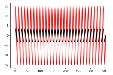
Step 1: Going back to the tide example that we showed in Week 12, create two pure sine
signals (ssh, ssh1) with the same period (12 hours) and phase
(\(0\ ^{\circ}\), but different amplitudes (15 cm and 3.4 cm).
Consider a length of 15 days.
import matplotlib.pyplot as plt

a = 15 # amplitude 1
a1 = 3.4 # amplitude 2
phase = 0
period = 12
omega = (2*np.pi/period) # convert period to rad

t = np.arange(0, 15*24+1, 1) # define time

# calculate the sine signals
ssh  = a*np.sin(omega*t - phase) # first ssh
ssh1  = a1*np.sin(omega*t - phase) # first ssh

# plot thw two waves

plt.plot(ssh, 'r-')
plt.plot(ssh1, 'k-')

plt.show()
Step 2: Using your pearson_corr() function, calculate the
correlation coefficient between ssh and ssh1.
r_ssh = pearson_corr(ssh, ssh1)

print("The correlation value between ssh and ssh is %f"%(r_ssh))
# The correlation value between ssh and ssh is 1.000000
Ok, so the correlation between them is maximum, i.e., 1. However, they are not really the same, right?
The Pearson correlation just tells us the relationship between two time series, or how they vary in relation to each other: if \(y\) increases (or decreases) at the same time that \(x\) increases (or decreases), then \(r = 1 (-1)\).
In some applications, for instance comparing model outputs to observed data, it is necessary to know more than this relationship. You also must know if they have the same magnitudes. How can we determine this?