The hydrostatic balance
You have already done this first part as an exercise week 5.
The pressure (\(P\)) in the athmosphere and in the interior ocean can be described in a first approximation as hydrostatic. The pressure (in the unit Pascal), that a particle located at the depth \(z\) in the ocean (where the surface has depth \(0\)) is subjected to is described by the following equation:
where \(\rho\) is the water density (with the unit \(\text{kg} \cdot \text{m}^{-3}\)), \(g\) is the acceleration of gravity (with the unit \(\text{m} \cdot \text{s}^{-2}\)) and \(z\) is the depth of the particle (with the unit \(\text{m}\)). The SI-unit for pressure is Pascal \([\text{Pa}]\), but in Meteorology and Oceangraphy pressure is usually presented in the unit decibar \([\text{dbar}]\). These to correspond according to the formula: \(1\,\text{Pa} = 10^{-4}\,\text{dbar}\).
We write function called hyd_pres() that calculates the pressure at a given
depth in the unit \(\text{dbar}\). The arguments of the function are: a
density value (\(\rho\)), the acceleration of gravity (\(g\)) and the
depth (\(z\)).
def hyd_pres(dens, g, z):
    P = -dens * g * z  # calculate pressure in Pa
    P = P / 1e4  # convert to dbar
    return P

#define constants
g = 10 # [m s-2]
dens = 1025 # [kg m-3]

#calculate the hydrostatic pressure at 100 m
hydP100 = hyd_pres(dens,g,-100)

print("The pressure is %f dbar"%(hydP100))
This gives us the following output:
The pressure is 102.500000 dbar
We will now investigate a bit more about this topic. First things first, let’s understand the physics behind it.
Fluid mechanics is the core of dynamical Oceanography and Meteorology. As such, this field is concerned to describe and reproduce the motion of fluids, such as water and air. The set of equations that describe how forces act on the fluid to put it in motion is known as the Navier-Stokes equations and it is directly derived from Newton’s second law: \(F = m\, a\), where \(F\) is the force applied in the studied object (\(N\)), \(m\) is the object mass (\(kg\)) and \(a\) is its acceleration (\(m\, s^{-2}\)).
We can decompose the various forces into the 3D reference frame with coordinates \(x\), \(y\) and \(z\). \(x\) and \(y\) represent the horizontal plane such as the land or ocean surface and \(z\) represents the vertical axis upward into the atmosphere or downward into the ocean interior. Here, we will focus on the vertical axis, and explore a simple and useful force balance called hydrostatic balance.
The hydrostatic balance is a strong assumption in geophysical fluid flows and it describes the balance between the gravity force (pointing downwards) and the gradient pressure force (pointing upwards). In the ocean, one can imagine it as the weight of the water column felt by a particle located at a certain depth. Such a balance is expressed by:
where \(g\) is the acceleration of gravity (\(m\, s^{-2}\)), \(\rho\) is the water density (\(kg\, m^{-3}\)) and \(\frac{dP}{dz}\) is the pressure gradient (\(Pa\, m^{-1}\)). To find an expression for pressure at a given depthin the ocean (we call this depth \(z_1\)), we can integrate the equation with respect to \(z\) from \(z_1\) to the ocean free surface (\(z_{surf}\)):
Air is much lighter than water, and we may therefore assume that the pressure at the ocean surface is negligible compared to the pressure in the ocean interior. This assumptions yields \(P(z) \sim 0\), for \(z \rightarrow\) \(z_{surf}\). We can also express the difference in depth between the surface and \(-z_1\) as \(\delta z\). If we regard \(z_{surf}\) to be zero, \(\delta z\) will be the same as the depth you are seeking the pressure for.
We are now left with a simple formula for hydrostatic pressure at the given depth \(z\):
This is the same equation that you manipulated in the previous assingment.
Task 1:
Given the hyd_pres function that we created before, calculate the pressure
from \(z = 0\) to \(z = -1000\) in increments of \(10\; m\). How
much does the pressure increase for every \(10\; m\) depth? Consider
\(\rho = 1025\; kg\, m^{-3}\) and \(g = 10\; m\, s^{-2}\).
(Hint: Start by making a depth array with the Numpy linspace function.)
## Task 1

# import necessary toolboxes
import numpy as np

#define constants
g = 10 # [m s-2]
dens = 1025 # [kg m-3]

# create array with depths every 10m
z_depths = np.linspace(0, -1000, 101)
# alternatively you can use np.arange
# z_depths=np.arange(-1000.,0.,10)

#calculate the hydrostatic pressure at each depth, assuming constant density
hydP1 = hyd_pres(dens, g, z_depths)

mean_diff = np.mean(np.diff(hydP1))

print("For every 10m, the pressure increases by %f dbar"%(mean_diff))
We get the following result:
For every 10m, the pressure increases by 10.250000 dbar
In other words, you increase the pressure by aroud \(10\; dbar\) for every \(10\; m\) deeper in the ocean. If you transfer this result to a more concrete example, the pressure we feel at the ocean surface is \(1\; atm = 10\; dbar\). You would experience \(100\) times more pressure at \(100\; m\) depth in the ocean in comparison to when you are at the surface!
Task 2:
a) Calculate the pressure at \(100\; m\) depth for density values ranging from \(0\) to \(1025\; kg\, m^{-3}\). (Tip: use the Numpy ’arange’ function.)
b) What is the mean rate of pressure increase for every \(\delta \rho = 5\; kg\, m^{-3}\)?
c) Is the pressure increase constant?
## Task 2
dens2 = np.arange(0, 1025 + 5, 5)

# a)
hydP2 = hyd_pres(dens2, g, -100)
# print(hydP2)

# b)
pres_incr = np.diff(hydP2)
mean_inc = np.mean(pres_incr)
print("The mean rate of pressure increase is %f dbar" % (mean_inc))

# c)
all_same = np.all(pres_incr == pres_incr[0])
if all_same:
    print("The pressure increase is constant.")
else:
    print("The pressure increase is not constant.")
We get the following output.
The mean rate of pressure increase is 0.500000 dbar
The pressure increase is constant.
Task 3:
The file zpd_file.txt contains pressure, temperature and salinity
values obtained from the Levitus 94 dataset in the coordinates
12.5\(^{\circ}\)S and 30.5\(^{\circ}\)W. The Levitus dataset
gathers data from different sources (research institutes), field campaings and
variables (temperature, salinity, oxygen and nutrients). All of this data
receives a quality control check and processing procedures before they are made
available to the community.
We will compare the pressure and density values obtained by using the
hydrostatic balance function hyd_pres that we created before with the
pressure and density data contained in the zpd_file.txt.
a) First of all, we open the file using the Pandas function read_csv
with column separator sep = r'\s+’. We define the variables df_z,
df_p and df_d. These variables will store the depths, pressure and
density values present in the zpd_file.txt.
## Task 3
import pandas as pd

#read the data into a pandas dataframe
df = pd.read_csv('zpd_file.txt', sep=r'\s+')

df_z = df.depth
df_p = df.press
df_d = df.dens
b) By using the hyd_pres function, we calculate the pressure for the
depths present in the file (df_z). Since density is a required
parameter in the function, use the first value of df_d as the
argument.
#calculate the hydrostatic pressure from the Levitus dataset. df_d[0] is the surface density
p_hyd = hyd_pres(df_d[0], g, df_z) # use the function

print(p_hyd)
We get the following output:
0       -0.000000
1       10.238348
2       20.476697
3       30.715045
4       51.191742
5       76.787612
6      102.383483
7      127.979354
8      153.575225
9      204.766966
10     255.958708
11     307.150449
12     409.533932
13     511.917415
14     614.300898
15     716.684381
16     819.067864
17     921.451347
18    1023.834830
Name: depth, dtype: float64
c) We compare this result with the observed pressure df_p. How much
do they differ?
#calculate the difference from the pressure given in the dataset
dif_p = p_hyd - df_p # make the difference

print(dif_p)
We get the following result:
0     -0.000000
1      0.176081
2      0.351712
3      0.526892
4      0.875902
5      1.309629
6      1.740539
7      2.168632
8      2.593905
9      3.435990
10     4.266789
11     5.086293
12     6.691385
13     8.251207
14     9.765696
15    11.234793
16    12.658436
17    14.036563
18    15.369112
dtype: float64
Ok, so we have essentially a difference of 0-15% between our values estimated with the hydrostatic balance assumption and the observed ones. Why do you think the differences are not the same throughout the water column?
Task 4:
a) We have been assuming so far that the density is constant throughout the water column (or atmosphere), but in fact it also varies with depth, i.e., \(\rho\) is a function of \(z\). Now, instead of finding pressure, let’s do it the other way round: use pressure values, depth levels and the acceleration of gravity to estimate densities.
For this, we need to use an interactive method.
Step 1: Create the lists d_hyd and d_o containing the first
observed density value from df_d as an initial item. For each
interaction in the loop, the new values of density will be stored in
these lists.
d_hyd = [df_d[0]] # to store density values calculated from p_hydrostatic
d_o = [df_d[0]] # to store density values obtained from the dataset
Step 2: Create the empty lists dp_dz_h (pressure from hydrostatic
balance) and dp_dz_o (pressure from file). These are the lists where the
\(\frac{dP}{dz}\) and \(dz\) values will be saved.
dp_dz_h = [] # rate of change of p_hydrostatic w.r.t z
dp_dz_o = [] # rate of change of p_observed w.r.t z
Step 3: Create the function diff_dp_dz, which takes as arguments the
pressure, the water depth and the list that the rates will be stored. This
function will calculate the rate of change of pressure (\(\frac{dP}{dz}\))
with respect to \(z\). For example, using the first two values provided in
the zpd_file.txt:
where \(i\) is every step in your list (in our case, variables in Task 3
have length 19 so \(i\) ranges from \(0\) to \(18\)). Use the
\(z\) depths provided in the zpd_file.txt.
Tips: Use a for loop within the diff_dp_dz ranging from \(0\) to
\(17\). We can’t loop til the last point (\(i = 18\)) because there is
no further values beyond it (\(i+1\), in the previous example). Use the
function append to store the values in the dp_dz_(h,o) lists. If you
struggle with the differentiation, try the function np.diff from Numpy.
def diff_dp_dz(p, z, lst):
    for i in range(0, len(df_p)-1):
        dp = p[i+1] - p[i] # diff p
        dz = z[i+1] - z[i] # diff z
        dpdz = dp/dz # take the rate

        lst.append(dpdz) # store value
    return

diff_dp_dz(p_hyd, df_z, dp_dz_h)
diff_dp_dz(df_p, df_z, dp_dz_o)
We have halfway done. To summarize, we calculated \(\frac{dP}{dz}\)
from Equation 1 for pressure values obtained with the hyd_pres
function and for the observed ones provided in the file.
Now, create the function dens_from_pres taking as arguments
\(\frac{dP}{dz}\), \(g\) and the list where the calculated density
values will be stored (d_hyd and d_o). Based on the hydrostatic balance,
this function must provide the calculated density values given \(P\),
\(z\) and \(g\). To clarify how the interactive method works, let’s
expand Eq. 1 as:
So, the new value of density (\(\rho (i+1)\)) is given by the density at the water depth above (\(\rho(i)\)) minus the rate of change of pressure between the two levels (\(\frac{dP}{dz}\)) and divided by the acceleration of gravity (\(g\)).
To make it work, use again a for-loop within the dens_from_pres function
ranging from \(0\) to \(17\). For each interaction (i+1), you must
access the density (d_hyd, d_o) and dp_dz (dp_dz_h, dp_dz_o)
values stored in the previous time steps (i), make the correct arithmetic
provided by Eq. 2 and store the new density value in the same density list.
d_hyd = [df_d[0]] # density values calculated from p_hydrostatic
d_o = [df_d[0]] # density values obtained from the dataset


def dens_from_pres(dpdz, g, den):
    for i in range(0, len(dpdz)):
        dens = den[i] - (1/g)*(dpdz[i])
        den.append(dens)
    return

dens_from_pres(dp_dz_o, g, d_o)
dens_from_pres(dp_dz_h, g, d_hyd)
b) Ok, so now we have density values calculated from pressure
obtained by using the hyd_pres function and from the data file!
As a next step, we calculate the difference between d_o and d_hyd.
# difference between estimated values
diff_dens = np.array(d_hyd) - np.array(d_o)

print(diff_dens)
We get the following output:
[0.         0.00176081 0.00351712 0.00526892 0.00701397 0.00874888
 0.01047252 0.01218489 0.01388598 0.01557015 0.01723175 0.01887076
 0.02047585 0.02203567 0.02355016 0.02501926 0.0264429  0.02782103
 0.02915358]
The difference between them is actually really small (around 0.1% to 3%).
c) As the last example, we calculate the difference between the observed
density values (df_d) and (d_o, d_hyd). Plot the estimated (d_o)
and observed (df_d) densities with Matplotlib.
import matplotlib.pyplot as plt

# difference between observed density and the estimated ones
diff_o_hyd = df_d - np.array(d_hyd)
diff_o_o = df_d - np.array(d_o)

plt.plot(df_d, df_z, 'r--', label='Observed')
plt.plot(d_o, df_z, 'k-', label='Estimated')

plt.xlabel('Density [kg m-3]')
plt.ylabel('Depth [m]')

plt.legend(loc='upper right')
plt.show()
We get the following plot:
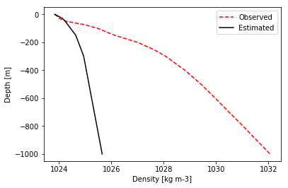
Why are they so different?