Land or Water? - numpy with large datasets

Let’s look at how we handle large data sets in numpy. As an example, we’ll take a world map at 1km resolution per pixel.

Dataset

The example data comes from (the now closed) http://www.landcover.org/data/landcover/. The University of Maryland Department of Geography generated this global land cover classification collection in 1998. Imagery from the AVHRR satellites acquired between 1981 and 1994 were analyzed to classify the world’s surface into fourteen land cover types at a resolution of 1 km 1 .

Download

First, let’s get all files we need, then we’ll discuss them afterwards. Create a new empty directory to work in, and…

• Download landcover.zip and extract the data file from it. It is called gl-latlong-1km-landcover.bsq and should be 933120000 bytes big. Put the unzipped data file in your working directory. This is a raw binary file of data, with no internal description of how we can interpret it. Nowadays, one would use a self-describing format such as NetCDF for this kind of geographical data.

• The data format is described in a separate file gl0500bs.txt (click to download).

  Information
  Image Size:                 43200 Pixels 21600 Lines
  Quantization:               8-bit unsigned integer
  Output Georeferenced Units: LONG/LAT E019
  Projection:                 Geographic (geodetic)
  Earth Ellipsoid:            Sphere, rad 6370997 m
  Upper Left Corner:          180d00'00.00" W Lon  90d00'00.00" N Lat
  Lower Right Corner:         180d00'00.00" E Lon  90d00'00.00" S Lat
  Pixel Size (in Degrees):    0.00833 Lon 0.00833 Lat
  (Equivalent Deg,Min,Sec):   0d00'30.00"0d00'30.00"
  UpLeftX:                    -180
  UpLeftY:                    90
  LoRightX:                   180
  LoRightY:                   -90
  

  We’ll make sense of it later. For now, let’s note the first 2 lines: it’s meant to be an image of 21600 lines with 43200 pixels. And the values are stored as 8-bit unsigned integer.

• The possible integer values go from 0 to 13, as we can see in the encoding of the land types mentioned on the project’s website: landcover_legend.png (click to download)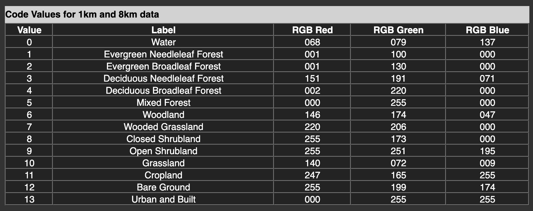

  

Making sense of it

What is actually in the data file? A search for «numpy load binary data» suggests numpy.fromfile. Let’s try it:

import numpy as np
data = np.fromfile('gl-latlong-1km-landcover.bsq')

print('data', data)
print('minmax', data.min(), data.max())
print('shape', data.shape)

We get:

   data [0.00000000e+000 0.00000000e+000 0.00000000e+000 ... 1.22416778e-250
1.22416778e-250 1.22416778e-250]
   minmax 0.0 8.309872195179385e-246
   shape (116640000,)

The values here make no sense. What has gone wrong? We were expecting integer values in the data file, but got very small float values instead. Also, from a file of size 933120000, we only got 116640000 values. We must be misinterpreting the binary data.

Let’s look at the documentation of np.fromfile We see that there is a dtype parameter we can specify, to determine the data type. By default it is float, which in Python is a 64-bit data type. So we are taking 64 bits from the file and interpreting them as a float number. Instead, the description told us it was 8-bit unsigned integer. In numpy, this is represented as uint8 (see numpy basic types)

Let’s try to specify this explicitly:

import numpy as np
data = np.fromfile('gl-latlong-1km-landcover.bsq', dtype='uint8')

print('data', data)
print('minmax', data.min(), data.max())
print('shape', data.shape)

The result is a lot better:

data [ 0  0  0 ... 12 12 12]
minmax 0 13
shape (933120000,)

We see that the values are integers, and they go from 0 to 13 like we expect. Only the shape is still strange. It should be 2-dimensional with 43200 pixels and 21600 lines. Instead, we have a one-dimensional long array with 933 million values. But \(43200\times 21600=933120000\)!

Let’s reshape the array into the right form:

data = np.fromfile('gl-latlong-1km-landcover.bsq', dtype='uint8')
data = data.reshape(21600, 43200)

Now the output is the right shape:

data [[ 0  0  0 ...  0  0  0]
 [ 0  0  0 ...  0  0  0]
 [ 0  0  0 ...  0  0  0]
 ...
 [12 12 12 ... 12 12 12]
 [12 12 12 ... 12 12 12]
 [12 12 12 ... 12 12 12]]
 minmax 0 13
 shape (21600, 43200)

Each position in the array approximately corresponds to a 1km x 1km square on Earth. The value at that position represents the dominant landcover.

Visualisation

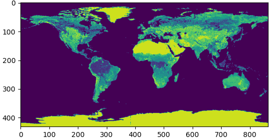
Remember that we can use plt.imshow() to look at 2-dimensional arrays. Let’s try that here. Viewing almost 1GB of data will be very resource-intensive. So let’s do a subsample of the data. We go from beginning to end in steps of 50: ::50. This will reduce the data size for plotting by \(50\times 50=2500\) to approximately 400kB:

viz_data = data[::50, ::50]

import matplotlib.pyplot as plt
plt.imshow(viz_data)
plt.show()

The result looks promising:

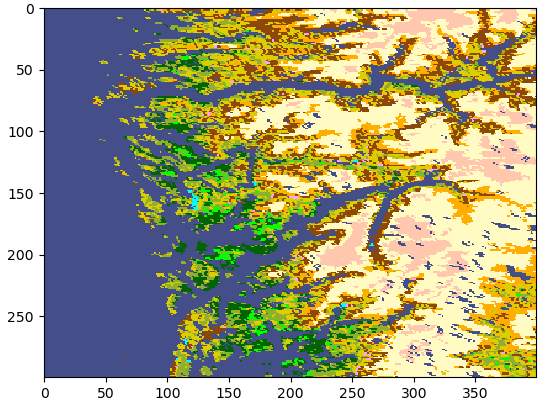
We can also use the original data set, as long as we don’t try to plot it all at the same time. Try these two alternatives. The last one nicely shows how detailed the data set is:

plt.imshow(data[2000:7000, 20000:25000])

plt.imshow(data[3400:3700, 22120:22520])

Colours

In the default colour scheme, it is hard to tell apart water from forest. Instead, let us use the RGB colour values given in the overview table:

In maptlotlib, we can use this information to create a colour map. Googling how to do this points us at some examples. Let’s look at the completed code:

import numpy as np
import matplotlib.pyplot as plt
from matplotlib import colors

rgb_colors = np.array([
        ( 68,  79, 137),
        (  1, 100,   0),
        (  1, 130,   0),
        (151, 191,  71),
        (  2, 220,   0),
        (  0, 255,   0),
        (146, 174,  47),
        (220, 206,   0),
        (255, 173,   0),
        (255, 251, 195),
        (140,  72,   9),
        (247, 165, 255),
        (255, 199, 174),
        (  0, 255, 255),
])/255  # matplotlib expects values from 0 to 1, so we divide by 255

landcover_cmap = colors.ListedColormap(rgb_colors)

data = np.fromfile('gl-latlong-1km-landcover.bsq', dtype='uint8')
data = data.reshape(21600, 43200)

bergen = data[3400:3700,22120:22520]
plt.imshow(bergen, cmap=landcover_cmap, interpolation='none')

plt.show()

Memory mapping

Maybe you noticed that np.fromfile takes a little while to load up the data set. The whole 1GB is copied into memory immediately.

We have an alternative, np.memmap, where the data is left on disk, and only loaded when it is needed. The syntax is very similar:

data = np.memmap('gl-latlong-1km-landcover.bsq',
                 mode='r',
                 shape=(21600,43200)
                )

We can directly specify the shape here. The option mode='r' makes the file read-only. If we do not set this, any changes we make to data will be immediately changed in the file, too!

The rest of the program can stay unchanged, but should run faster now if we don’t use all the data points.

References

1

Hansen, M., R. DeFries, J.R.G. Townshend, and R. Sohlberg (1998), UMD Global Land Cover Classification, 1 Kilometer, 1.0, Department of Geography, University of Maryland, College Park, Maryland, 1981-1994.

Hansen, M., R. DeFries, J.R.G. Townshend, and R. Sohlberg (2000), Global land cover classification at 1km resolution using a decision tree classifier, International Journal of Remote Sensing. 21: 1331-1365.