Tides and the sea level
Background
Tidal oscillations originate from the gravitational interactions between the Earth and other celestial bodies, especially the Sun and the Moon. variations in the sun and the moon position relative to the Earth, give rise to periodic motions with different frequencies. You can think of the total tides as the sum of many waves with slightly different frequencies (\(\omega\)), amplitudes (A) and phases (\(\phi\)). Consider the following sine wave equation and Figure 1 below:
A: This is the magnitude of the wave. If you keep all the other parameters fixed but change the amplitude (A\(_{1}\) = 1, A\(_{2}\) = 0.5), you will obtain the waves in the top-left panel in Figure 1.
\(\omega\): This is the frequency (which is the inverse of the period: \(T = \frac{1}{f}\)) of the wave. It represents how many cycles of the signal are present in a given amount of time (say 1 second). If a signal Y1 has higher frequency (or lower period) than Y2, it means that Y1 presents more crests and troughs than Y2. Using the equation above, if you fix the other parameters but change the frequency (\(\omega_{1} = 2 \pi\), \(\omega_{2} = 4 \pi\)), you will get the waves in the bottom-left panel in Figure 1. Since \(\omega_{2}\) is twice \(\omega_{1}\), you get the double amount of crests and troughs per unit of time.
\(\phi\): This is the phase of a wave. It represents the ‘position’ of the wave features (crests, troughs, ascending or descending motion) in time or space. For example, if you take a pure sine wave \(y = \text{sin}(x)\) (where \(\phi = 0\)), the crests occur when \(x\) takes the values \(\pi\), \(2\pi\), \(4\pi\), \(6\pi\), and so on. If you change \(\phi\) to \(\frac{2}{\pi} \; \text{rad}\) (so that \(y = \text{sin}(x - \frac{\pi}{2}\))), you will shift your signal by this angle, so the crests will now occur when \(x\) takes the values \(\frac{\pi}{2}\), (\(2\pi+\frac{\pi}{2}\)), (\(4\pi+\frac{\pi}{2}\)), (\(6\pi+\frac{\pi}{2}\)), and so on. Two waves are said to be in phase, if their crests and troughs are occur at the same \(x\)-values. If there is an offset between them, they are out of phase. Going back to our y\(_{1}\) and y\(_{2}\) signals, keeping the other parameters constant but considering \(\phi_{1}\) = 0 and \(\phi_{2}\) = \(\frac{\pi}{6}\) give us the waves in the top-right panel in Figure 1. These waves are out of phase.
The bottom-right panel in Figure 1 below shows our y\(_{1}\) and y\(_{2}\) waves when all the changes made before are applied at once.
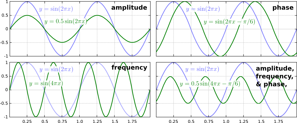
Figure 1: Comparison of different sine waves.
source: https://www.pngkey.com/maxpic/u2w7e6q8o0u2i1y3/
These single waves are often referred to as tidal constituents, and their frequencies/periods are known accurately from astronomical calculations. Although we are aware of hundreds of constituents, we usually only need about ten of them to describe more than 90% of the observed tidal variation.
The tides are visible through changes in the sea surface height SSH. When we make observations of SSH as a function of time (\(t\)), we measure a combination of the local mean sea level (\(H\)) and the influence of tides \(\text{Ti}(t)\). In addition, there could be influence from meteorological forcing \(\text{M}(t)\), such as wind/storms.
In this example, we will investigate some properties of tides and compare a pure tidal signal to observed sea level measurements.
Data
The amplitudes and phases of tidal constituents vary from place to place, due to interference with land masses (the waves will have to travel around the land masses). Table 1 provides amplitudes, periods and phases for 6 components (M2, S2, N2,K2, O1 and K1) obtained at Kartverket from sea level observations in Stavanger.
Component |
Amplitude [cm] |
Period [hours] |
Phase [deg] |
|---|---|---|---|
M2 |
15.85 |
12.42 |
0.33 |
S2 |
6.68 |
12.00 |
6.18 |
N2 |
2.59 |
12.66 |
1.00 |
K2 |
1.19 |
11.97 |
0.33 |
O1 |
1.50 |
25.82 |
5.85 |
K1 |
5.44 |
23.93 |
5.44 |
Table 1: data for 6 tidal constituents.
M2: Principal semi-diurnal lunar component;
S2: Principal semi-diurnal solar component;
N2: Larger lunar elliptic component;
K2: Lunisolar semi-diurnal component;
O1: Principal diurnal lunar component;
K1: Diurnal declination component;
For more information about tides, check the compendium developed by Prof. Helge Drange here.
Task 1
Given the values in Table 1, we create the dictionary comps
containing the tidal components as keys and amplitude, period and
phase as their corresponding values. (It is important to remember to keep the
same order in every entry.)
# comps = {'m2':[A, Pd, Ph], 's2':[], ... }

comps = {'m2':[15.85,12.42,0.33], 's2':[6.68,12.00,6.18], 'n2':[2.59,12.66,1.00],\
         'k2':[1.19,11.97,0.33], 'o1':[1.50,25.82,5.85], 'k1':[5.44,23.93,5.44]}
Task 2
We create the dictionary tides, with the same keys as comps but with
empty lists as entries.
# tides = {'m2':[], 's2':[]...}
tides = {'m2':[], 's2':[], 'n2':[], 'k2':[], 'o1':[], 'k1':[]}
Task 3
We create the function elev that takes as arguments the name
of the tidal component and its wave parameters. By using a cosine
function, we calculate the SSH associated to each of the components for 45
days. Then we save the calculated tidal elevation in the corresponding key
within the tides dictionary.
Tip: Period must be converted to radians. The period in radians, \(T_{\text{rad}}\), is given by \(T_{\text{rad}} = \frac{2 \pi}{T_{\text{deg}}}\), where \(T_{\text{deg}}\) is the period in degrees.
Tip 2: Import the Numpy library and use the cosine function.
import numpy as np

#def elev(td, period, amplitude, phase, time):
    #omega =  # convert period to rad

    #ssh  =  # calculate sea level elevation with a cosine wave equation
    #tides[td].append(ssh)

def elev(td, period, amplitude, phase, time):
    omega = (2*np.pi/period) # convert period to rad

    ssh  = amplitude*np.cos(omega*time - phase) # calculate sea level elevation with a cosine wave equation
    tides[td].append(ssh) # append the elevation time series on the corresponding *tides* key

t = np.arange(0, 45*24+1, 1) # 45 days
[elev(i, comps[i][1], comps[i][0], comps[i][2], t) for i in tides.keys()]
The dictionary tides now looks like this:
{'m2': [array([14.99477114, 15.60544637, 12.30671726, ..., -0.69987822,
          7.06102109, 13.05302602])],
 's2': [array([6.64446987, 5.41025202, 2.72636152, ..., 3.91810835, 6.09830738,
         6.64446987])],
 'n2': [array([1.39938297, 2.26833165, 2.58992917, ..., 2.58578986, 2.34410462,
         1.53678411])],
 'k2': [array([1.12579039, 1.16746723, 0.89478839, ..., 1.18916615, 1.0067461 ,
         0.55324662])],
 'o1': [array([1.36144992, 1.169624  , 0.90887743, ..., 0.63461137, 0.94340083,
         1.19659995])],
 'k1': [array([ 3.61807615,  2.43964282,  1.09398337, ...,  2.24630069,
          0.88331309, -0.5402215 ])]}
Plotting
Let’s sum up all of the components and make a simple plot:
import matplotlib.pyplot as plt

ssh = tides['m2'][0] + tides['s2'][0] + tides['n2'][0] + tides['k2'][0] + tides['o1'][0] + tides['k1'][0]

plt.plot(ssh);
labels = np.linspace(0, 45, 24*45+1)
plt.xticks(t[0:-1:24*7], labels[0:-1:24*7], rotation=45); # change xticks to days

plt.xlabel('Days')
plt.ylabel('SSH (cm)')
plt.show()
We get the following plot:
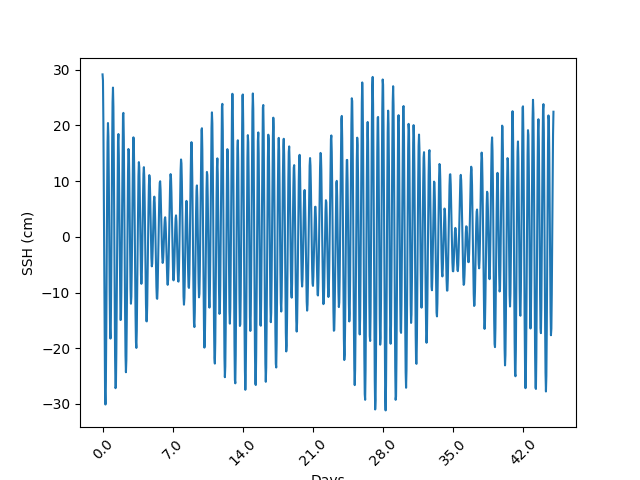
PS: The signal presents a clear 14 days period modulation. Why does this happen?
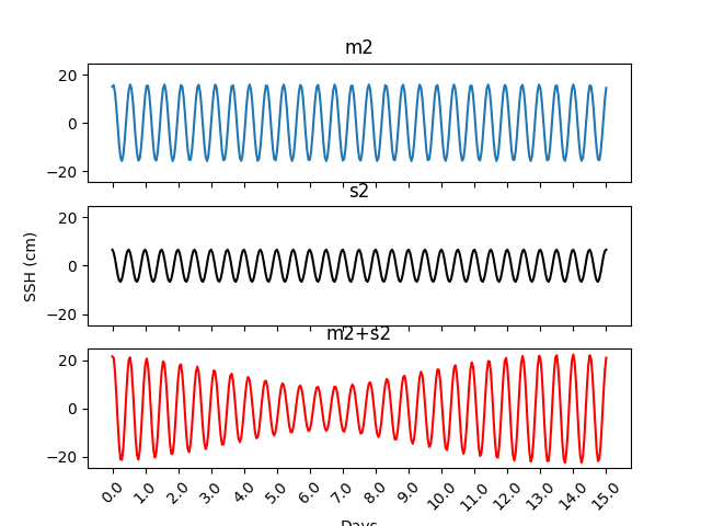
Lastly, let’s plot two components (M2 and S2) for 15 days and check how
they look like when they are superimposed. To do this, we sum the two
components of interest using the variable sum_tides.
#sum_tides = tide1 + tide2
sum_tides = tides['m2'][0]+tides['s2'][0]

fig, (ax0, ax1, ax2) = plt.subplots(nrows=3, ncols=1, sharex=True, sharey=True)

ax0.plot(tides['m2'][0][0:15*24+1]) #m2 component
ax0.set_title('m2')

ax1.plot(tides['s2'][0][0:15*24+1], 'k-') #o1 component
ax1.set_title('s2')

ax2.plot(sum_tides[0:15*24+1], 'r') #superimposed component
ax2.set_title('m2+s2')

plt.xticks(t[0:15*24+1:24], labels[0:15*24+1:24], rotation=45); # change xticks to days

plt.xlabel('Days')
ax1.set_ylabel('SSH (cm)')
plt.show()
This gives us the following plot: